Solved! North American Domain RAP 13.5km Rotated Pole GRIB2 for GIS
Posted: September 10, 2019
Valuable Weather Model Forecast Data Finally Available to Global Geo Community after Cracking Technical Puzzle
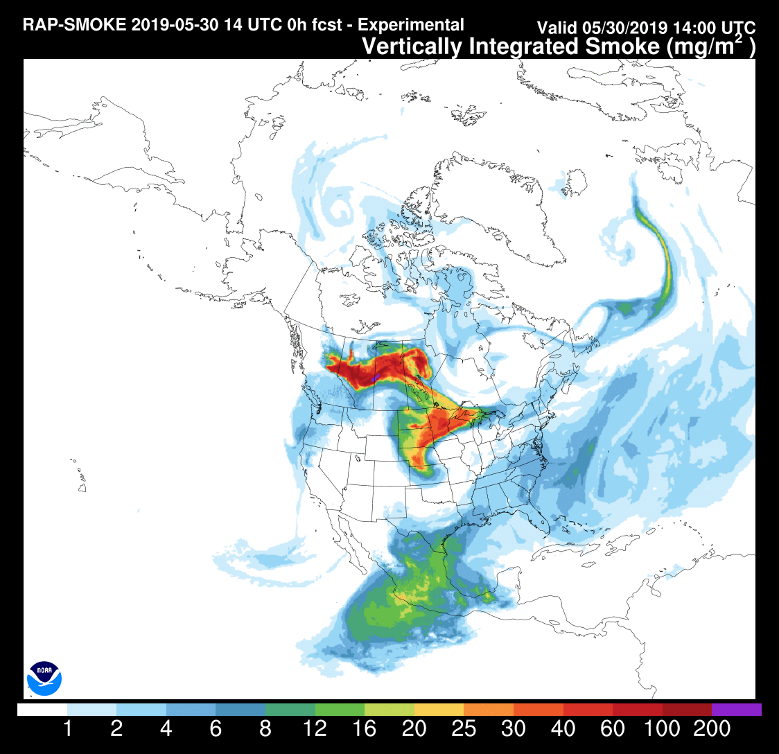
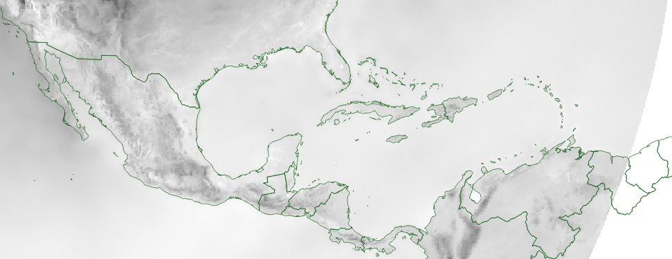
Figure 1. Example of the area of coverage and spatial extent of the North American domain for RAP Smoke Forecasts. Coming soon to RealEarth.
Many researchers in the Earth sciences have been frustrated with the difficulty of mapping Rapid Refresh (RAP) model output from NOAA’s National Centers for Environmental Prediction (NCEP) in GIS (Geographic Information Systems). Here’s the good news: we now have a way to do that for the 13.5km resolution North American domain (Figure 1) using the recently updated standard libraries: PROJ v6.x, GDAL v3.x. Why does this matter? Because as research in the atmospheric sciences begins to converge with research in the earth sciences, technical barriers to data sharing still exist that inhibit innovation and collaboration. This solution removes one of those barriers. It gives practitioners of GIS a way to access model output from the North American domain of the RAP using their tools in their familiar computing environment. — Sam Batzli, CIMSS/SSEC, University of Wisconsin-Madison
Acknowledgement
I’ve been working on this problem off and on for a few months. I reached out to Kevin Sampson at UCAR because I came across some code he had written to try to address this problem. We exchanged examples, tests, and thoughts in a series of emails, each time inching closer to a solution. We could not have solved this problem without working together. The same is true of Eric James, a NOAA affiliate at the Earth System Research Lab (ESRL) involved in putting smoke forecasts into the RAP output (raw data is still experimental and not yet distributed publicly). He introduced me to the software packages wgrib2 and NCL (NCAR Command Language) and provided unpublished domain parameters that confirmed our ultimate solution.
Background
My entry into this puzzle came via a request from the JPSS-PGRR (Joint Polar Satellite System Proving Ground and Risk Reduction), Fire and Smoke Initiative to put hourly smoke forecasts from the RAP North American full domain into our visualization platform “RealEarth.” “No problem,” I though. “It will be as easy as it was to put in the HRRR CONUS smoke forecasts that we’ve been doing now for over a year.” I was wrong. The problem stemmed from a basic incompatibility in describing geographic projections across academic disciplines.
The way the geographic extent and shape of the RAP full North American domain (also known as an “Arakawa staggered E-grid on rotated latitude/longitude grid”) is defined in the modeling environment is as an equidistant cylindrical projection (or Plate Carrée), in which the Earth (represented as a perfect sphere) has been rotated south such that the North Pole and entire arctic circle are visible as well as parts of Siberia, Northern Europe, Hawaii, and even parts of South America below the equator (see Figure 1). For weather modeling, there are distinct advantages to using an Arakawa grid. As noted in its Wikipedia entry, it offers a way “to represent and compute orthogonal physical quantities (especially velocity- and mass-related quantities) on rectangular grids used for Earth system models for meteorology and oceanography.” While there is nothing inherently wrong with representing the earth as a staggered grid on a rotated sphere, it is unconventional in the world of geodesy, geography, and GIS. Geographers in the earth sciences would usually construct maps like this with an Azimuthal Equidistant projection. The rotated pole approach (referred to by geographers as a general oblique transformation), works well in a modeling environment, but is seldom used by geographers because it depends on a spherical model of the earth (not the preferred and more accurate ellipsoid, WGS84) and involves two transformations (a cylindrical projection and a rotation). It simply was not, and still is not, fully supported in most GIS software. Furthermore, the full set of parameters needed by GIS to describe the “Arakawa staggered E-grid on rotated latitude/longitude grid” with 13.5km resolution, over North America have not been published in one place (until now). Skip to steps 4, 5, and 6 if you want to go straight to the answers.
Software packages and tools more commonly used in the atmospheric sciences such as MATLAB, the GEOGRID module within the Weather Research Forecast (WRF) Preprocessing System (WPS), Climate Data Operators (CDO), Generic Mapping Tools (GMT), wgrib2, and NCL offer partial or internal support for rotated pole projections. With the exception of maybe MATLAB, these are not commonly used in GIS environments. Further complicating the issue is the use of super efficient hierarchical and multidimensional data bundling formats such as GRIB2, HDF, and netCDF as the data output formats from the RAP and similar models. While GIS software is getting better at parsing the metadata for these formats, it draws a blank when encountering non-standard projections and descriptions of the earth, such as a rotated pole. So if you want to overlay data from RAP’s North American grid on data of the same geographic location in a GIS without installing and learning a whole new set of tools, it is not so easy.
Fortunately, the transformation software combination of PROJ and GDAL now can accommodate the notion of a “rotated pole.” Unfortunately additional steps are needed to translate the parameters of the rotated pole RAP North American Domain in terms understandable and expected by PROJ or GDAL. The rest of this post describes the steps that we took to make it work.
Describing the Projection in GIS-friendly Terms
Our goal here is to produce a GeoTIFF with a well defined projection that we can then reproject into something that GIS mapping software like QGIS and ArcGIS (that are currently built on older versions of GDAL and PROJ) can handle. So even when we correctly define the output GeoTIFF (which we do in Step 5 below), it will not work in GIS until future software versions incorporate the latest capabilities of GDAL and PROJ. So we apply an additional projection in Step 6 to make the GeoTIFF backward compatible.
Step 1: Get Some Example Data
First we need example data set to work with. Publicly accessible RAP model data is available here: ftp://ftpprd.ncep.noaa.gov/pub/data/nccf/com/rap/prod/rap.<yyyymmdd>/ (substitute today’s date for <yyyymmdd> or browse to a directory of your choice). I recommend logging in with “user:anonymous” and “password:<your email>” using an FTP client like FileZilla or command line utility like wget or curl to grab an example data set. Since the example data we want is in GRIB2 binary format, be sure to download with transfer type set to “binary.” If you are browsing in FileZilla, you will notice many files in the “prod” directory. Most are associated with specific AWIPS Grids (the closed software system used by the National Weather Service). Those files are subsets of the full North American domain, usually in a standard Lambert Conformal Conic projection that will already work in a GIS because their projection parameters are recognizable by a GIS, but what we want is an example file of the full RAP domain with the pattern “rap.t06z.wrfprsf02.grib2”. Translating this file name… “rap” is the name of the model implementation; “t06z” stands for the hour time step output of the model run in UTC/Zulu (there are 21, one-hour time steps in each model run; “wrfprs” stands for WRF model output with pressure levels, essentially comprising a vertical array of altitude levels, of the North American Domain for most of the variables; “f02” stands for the hour in UTC of the forecast run (the model is run every hour); and “grib2” is the output format.
>wget ftp://anonymous@ftpprd.ncep.noaa.gov/pub/data/nccf/com/rap/prod/rap.20190906/rap.t06z.wrfprsf02.grib2

or

>curl -u anonymous:<your_email> 'ftp://ftpprd.ncep.noaa.gov/pub/data/nccf/com/rap/prod/rap.20190906/rap.t06z.wrfprsf02.grib2' -o ~/Downloads/rap.t06z.wrfprsf02.grib2
I have only tested this methodology on the above public files and the not-yet-public experimental GRIB2 files that contain additional variables such as surface smoke, column integrated smoke. In theory, this approach will work for all GRIB2 output files for the “Arakawa staggered E-grid on rotated latitude/longitude grid” of 13.5km resolution, full North American domain with GRIB2 output files.
Step 2: E Pluribus Unum – Reading the Metadata and Extracting a TIFF
First, let’s see what we have. Running gdalinfo on the newly downloaded file will give us a summary. Be sure you are running the latest version (or 3.0 or above) of the GDAL tools. Earlier versions will not be able to read these GRIB2 files.
>gdalinfo --version
GDAL 3.0.1, released 2019/06/28
Now run gdalinfo with the -proj4 flag (proj was stuck at v4 for so long that it became part of the name for a while). The top of the output will look like this:
>gdalinfo -proj4 rap.t06z.wrfprsf02.grib2
Driver: GRIB/GRIdded Binary (.grb, .grb2)
Files: ../../Downloads/rap.t06z.wrfprsf02.grib2
Size is 953, 834
Coordinate System is:
GEOGCS["Coordinate System imported from GRIB file",
    DATUM["unknown",
        SPHEROID["Sphere",6371229,0]],
    PRIMEM["Greenwich",0],
    UNIT["degree",0.0174532925199433]]
PROJ.4 string is:
'+proj=longlat +a=6371229 +b=6371229 +no_defs '
Origin = (0.000000000000000,0.000000000000000)
Pixel Size = (0.000000000000000,-0.000000000000000)
Corner Coordinates:
Upper Left  (   0.0000000,   0.0000000) (  0d 0' 0.01"E,  0d 0' 0.01"N)
Lower Left  (   0.0000000,   0.0000000) (  0d 0' 0.01"E,  0d 0' 0.01"N)
Upper Right (   0.0000000,   0.0000000) (  0d 0' 0.01"E,  0d 0' 0.01"N)
Lower Right (   0.0000000,   0.0000000) (  0d 0' 0.01"E,  0d 0' 0.01"N)
Center      (   0.0000000,   0.0000000) (  0d 0' 0.01"E,  0d 0' 0.01"N)
Band 1 Block=953x1 Type=Float64, ColorInterp=Undefined
  Description = 0[-] MSL="Mean sea level"
...
Band 779 Block=953x1 Type=Float64, ColorInterp=Undefined
  Description = 0[-] NTAT="Nominal top of atmosphere"
...
So think of this as a data cube with multiple data layers representing one time-step of forecast output: four dimensions (latitude, longitude, altitude, and time). That is the beauty of GRIB2. It is a highly efficient ways to organize, store, and move a lot of information. Like other hierarchical science data formats such as HDF and NetCDF, it is essentially a self-contained and self-describing file-database. The difficulty with GRIB2 in the case of “wrfprs” and the full North American domain, is that until now you needed specialized software common only in the atmospheric sciences to crack it open. Even so, from my novice perspective, one needs a veritable blackbelt in wgrib2 or NCL software to get anything meaningful out. My goal is to allow people in the Earth sciences to use tools familiar to them and that are part of their workflow to access these important data sets.
From the “gdalinfo” command above we now have a definition of the sphere that is used in this version of the model: “+proj=longlat +a=6371229 +b=6371229 +no_defs” (“+a” is the equatorial radius and “+b” is the polar radius — since this is a sphere, this is the same +R=6371229, “+no_defs” instructs PROJ not to set default values for undefined variables). We can also see that the “Size is 953, 834”. These are the pixel dimensions of the raster layers in width and height. Other than that, gdalinfo really gives us nothing that will allow us to place this in geographical space. For example, gdalinfo does not recognize the existence of corner coordinates and therefore cannot calculate pixel size (spatial resolution) in this rotated pole GRIB2 file. So this data simply cannot be mapped by GDAL/PROJ and GIS software as is. We will have to turn to wgrib2 or NCL tools for help in collecting more parameters from the GRIB2 file.
Fun fact: the UNIT[“degree”,0.0174532925199433]] is the standard definition of a degree. It is calculated by dividing Π (pi) by 180 radians.
If you ran the gdalinfo command above, you will not doubt have noticed that there are 779 “Bands” or data sets within the GRIB2 file, and you had to scroll back up through all 11,730 lines to get to the top of the output just to see the general information info above. That’s a lot of information. Let’s simplify. Out of many bands, let’s extract one as a TIFF to see what it looks like. Using a suggestion from Kevin Sampson, we are going to extract the variable “TSOIL” (soil temperature) because unlike other variables like clouds or wind, TSOIL shows enough fixed geographic features and coastline elements that we can see what we are working with as we try to snap this data into geographic reality. From the gdalinfo above, we find that TSOIL is located as Band 628. Now let’s extract a TIFF (I’m giving it the name “unnav” because it is “un-navigated” which is a term atmospheric scientists and meteorologists use to mean it has no geographic coordinate system or defining information, it’s un-navigated or lost. Geographers would say that it is “not geolocated”).
>gdal_translate -b 628 rap.t06z.wrfprsf02.grib2 TSOIL_unnav.tifWe get a single band, 64-bit floating point TIFF. After playing with the contrast and scale in Photoshop and converting to a web-friendly PNG, it looks like this (Figure 2):
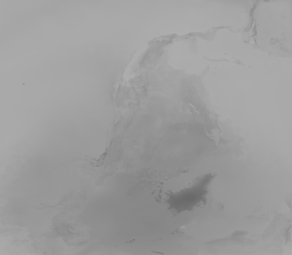
Figure 2: Raw output from RAP North American Domain. Notice that north and south are flipped.
Perhaps the first thing we notice is that this is a mirror image of what we were expecting for the North American domain as seen in Figure 1. The location of Greenland and faint outlines of the North American coastline shows that the data has a “south-up” rather than “north-up” orientation. It is unconventional, but not “wrong,” per se. No judging. We just note it and return to the blog, with gentle kindness. We can find joy and gratitude in the general dimensions and shape. These look good. Let’s press on.
Step 3: Squeezing Water from a Stone – Get Additional Parameters
We need more information. To define this projection in PROJ terms, we will use a general oblique transformation of a sphere-based equidistant cylindrical projection. The transformation command we want to use looks like this: >proj +proj=ob_tran +o_proj=eqc +o_lon_p=? +o_lat_p=? +lon_0=? +R=6371229. Therefore, for this part we need to know the location of the new pole (+o_lon_p=? +o_lat_p=?) and the center longitude of the resulting map (+lon_0=?). To make our output raster we will also need the latitude of the projection center and corner points. So for a complete definition of this grid in GIS-friendly format, we need a minimum of ten parameters (including a second version of the longitude of projection center that we will talk about later). From these, we will be able to make a GIS compatible GeoTIFF:
What we have so far:
- Type of transformation: +proj=ob_tran
- Type of initial projection. +o_proj=eqc
- Radius of the projection sphere +R=6371229
- Pixel dimensions of the raster: -outsize 953 834
Still need:
- New pole longitude: +o_lon_p=?
- New pole latitude: +o_lat_p=?
- Longitude of projection center: +lon_0=? (source)
- Longitude of projection center: +lon_0=? (target)
- Latitude of projection center: +lat_0=?
- Corner points (upper left, lower right) in projected units (meters): -a_ullr ulx? uly? lrx? lry?
After extensive poking around on the Internet and much consulting with Eric James, I obtained corner points that looked plausible. But I wanted to confirm those and have a more reliable way to get this info. On Eric’s suggestion, I turned to NCL and a tool called “ncl_filedump” (with the -c option for coordinate information), to dump more metadata about this domain to get the remaining four parameters that describe the rotated pole grid template. Doing so, I get the following:
>ncl_filedump -c rap.t06z.wrfprsf02.grib2
...
      float gridlat_0 ( ygrid_0, xgrid_0 )
         corners :	( -10.5906, -10.5906, 46.59194, 46.59194 )
         long_name :	latitude
         grid_type :	Arakawa Non-E Staggered rotated Latitude/Longitude Grid
         units :	degrees_north
         Dj :	0.121833
         Di :	0.1218331
         Lo2 :	22.66102
         La2 :	46.59194
         CenterLon :	254
         CenterLat :	54
         Lo1 :	220.9142
         La1 :	-10.5906

      float gridlon_0 ( ygrid_0, xgrid_0 )
         corners :	( -139.0858, -72.91415, 22.66102, 125.339 )
         long_name :	longitude
         grid_type :	Arakawa Non-E Staggered rotated Latitude/Longitude Grid
         units :	degrees_east
         Dj :	0.121833
         Di :	0.1218331
         Lo2 :	22.66102
         La2 :	46.59194
         CenterLon :	254
         CenterLat :	54
         Lo1 :	220.9142
         La1 :	-10.5906
Now we have official corner points in longitude-latitude. As longitude/latitude pairs we have four points: 1) -139.0858 -10.5906, 2) -72.91415 -10.5906, 3) 22.66102 46.59194, 4) 125.339 46.59194.
Step 4: Miracles and Magical Thinking – Logic and Luck – Trial and Error
With an oblique projection, it is difficult to know which point goes where unless you plot them as in Figure 3. Here we are using an Azimuthal Equidistant (defined by +proj=aeqd +lat_0=54 +lon_0=-106 +x_0=0 +y_0=0 +a=6371229 +b=6371229 +units=m +no_defs) as an approximation of the rotated pole North American domain, just to test out the corner and center points . Here’s what we see in QGIS: LL) -139.0858 -10.5906, LR) -72.91415 -10.5906, UR) 22.66102 46.59194, UL) 125.339 46.59194 Center) -106 54
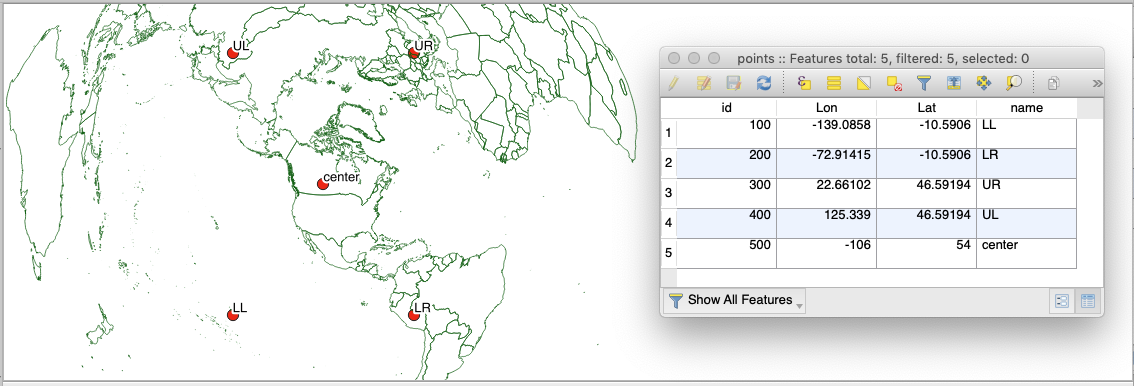
Figure 3. Mapping the corner and center points in an approximate projection (Azimuthal Equidistant) helps identify which point is which, in terms of upper, lower, left, and right.
To preserve our sanity as we dive into abstract reality, it is helpful to use magical thinking and consider these parameters in terms of “source condition,” or how the data are natively mapped (Figure 2) and “target condition,” or how it ultimately appears on the projected map (Figure 1). The points look great on the map in Figure 3, however we know our data is flipped, so here we need to describe the source condition in target terms and flip the latitudes, or y-values (only). Upper Left becomes Lower Left, and Upper Right becomes Lower Right like this: UL) -139.0858 -10.5906, LR) 22.66102 46.59194
Center Longitude is given as 254 and uses a 360 degree model of the world rather than the more conventional -180 to 180 around the Prime Meridian or “Greenwich.” Subtracting 360 from 254 gives us the more familiar -106 (west), which along with 54 (north) makes sense as a center point of our target condition when we look at Figure 3. To get the center of our projection to be at 54 degrees north rather than the equator (that would be the center latitude of the unrotated cylindrical projection), we have to rotate the Earth inside that cylinder to the south by 36 degrees (90-36=54). Continuing our magical thinking, we suspect that the latitude model is using 180 rather than the more conventional -90 to 90 and in our flipped source condition, we are recognizing that the latitude of north pole in this model is 0, the equator is 90 and the south pole is 180. Since the pole latitude is rotated by 36 degrees, let’s subtract 36 from 180, rotating 36 degrees north from the south pole (180-36=144). Since we don’t want to rotate the pole east or west and don’t know what else to do with it, we put our faith in our Higher Power and leave the source “New pole longitude” at a generic 180, with a willingness to change it to some other generic like 0 or 360 if necessary. It wasn’t necessary. This is the only mysterious parameter that I cant explain. 180 is the only thing that seems to do the trick in upside-down land. Perhaps the original south pole was defined as 180, 180 and since we are only doing an oblique rotation, this arbitrary longitude (since any longitude is valid for the pole of a sphere) remains the same. I welcome suggested explanations. From my correspondence with Eric James, I can confirm that it is indeed the value assigned to that parameter in the model input start-up file that launches RAP. [Spoiler alert for source longitude of projection center: its 74! I tried using Center Longitude as -106, but it didn’t work. I tried using 254 and that didn’t work either. I noticed that in one of our email exchanges my colleague Keven Sampson was attempting to use 74 and surmised that perhaps the longitude model maybe counting up to 360 in the other direction (…since the data are flipped, that actually makes boatloads of sense: 254-180=74). But if I hadn’t noticed what Kevin tried, I doubt I would have consider this and this blog post would not exist.]
So we now have all ten of our parameters, together in one place:
- Type of transformation: +proj=ob_tran (source)
- Type of initial projection. +o_proj=eqc (source)
- Radius of the projection sphere +R=6371229 (source)
- Pixel dimensions of the raster: -outsize 953 834 (target)
- New pole longitude: +o_lon_p=180 (source)
- New pole latitude: +o_lat_p=144 (source)
- Longitude of projection center: +lon_0=74 (source)
- Longitude of projection center: +lon_0=-106 (target)
- Latitude of projection center: +lat_0=54 (target)
- Corner points (upper left, lower right): -a_ullr -6448701.88 -5642620.27 6448707.45 5642616.94 (source)
“But wait,” you ask, “how did you get the corner points from lon/lat into x/y meters?” Good question! We transformed the points using PROJ with the other projection parameters… and a little bootstrapping …and some guesswork …and some more magical thinking. In its own words, “PROJ is a generic coordinate transformation software that transforms geospatial coordinates from one coordinate reference system (CRS) to another. This includes cartographic projections as well as geodetic transformations. PROJ includes command line applications for easy conversion of coordinates from text files or directly from user input.” It is in part what GDAL, and the internal workings of many GIS systems, use to manipulate rasters, pixel by pixel. We can use the command line application for our individual corner points.
I also found I could use this as a way to test and tune several of our transformation parameters described above. In the process of finding a solution for the center point, I essentially reverse-engineered the logic that produced the pole and center latitude and longitude parameters above. I tested various combinations of parameters using the general oblique transformation. My understanding is that an equidistant cylindrical projection generally maps a globe that is centered on lon/lat 0,0 onto a two-dimensional square in units of meters with a cartesian origin of 0,0 and extending outward with +/-northings on the y-axis and +/-eastings on the x-axis. So, I surmised that a correct center point for this rotated projection would also be 0,0. This turned out to be an important lucky-logical guess. After much trial and error, here are the commands and results:
>echo -106 54 | proj +proj=ob_tran +o_proj=eqc +o_lon_p=180 +o_lat_p=144 +lon_0=74 +R=6371229
0.00	0.00

>echo -139.0858 -10.5906 | proj +proj=ob_tran +o_proj=eqc +o_lon_p=180 +o_lat_p=144 +lon_0=74 +R=6371229
-6448701.88	-5642620.27

>echo 22.66102 46.59194 | proj +proj=ob_tran +o_proj=eqc +o_lon_p=180 +o_lat_p=144 +lon_0=74 +R=6371229
6448707.45	5642616.94
It is really great that GDAL 3.x recognizes and processes the general oblique transformation that PROJ describes. I believe that over time this will have a significant impact on data interoperability and collaboration across the Earth and atmospheric sciences.
Step 5: Extract a GeoTIFF from the GRIB2 and Apply the Projection Definition
>gdal_translate -b 628 -a_srs "+proj=ob_tran +o_proj=eqc +o_lon_p=180 +o_lat_p=144 +lon_0=74 +R=6371229" -outsize 953 834 -a_ullr -6448701.88 -5642620.27 6448707.45 5642616.94 /path/to/grib2/rap.t06z.wrfprsf02.grib2 /path/to/output/TSOIL_nav.tifSo all of this gets boiled down into one “gdal_translate” command. Maybe I should put this at the top.
Step 6: Reprojecting for Backward Compatibility with GIS
This step is necessary only until GIS software incorporates GDAL 3.x and PROJ 6.x. I’m choosing an Azimuthal Equidistant projection centered on -106, 54 as in Figure 3 so we can admire a similar looking projection in QGIS.
>gdalwarp -t_srs "+proj=aeqd +lon_0=-106 +lat_0=54 +x_0=0 +y_0=0 +a=6371229 +b=6371229 +units=m +no_defs" -dstalpha /path/to/TSOIL_nav.tif /path/to/output/TSOIL_aeqd.tif The final result looks like this (Figures 4 and 5) and shows an excellent fit to the Natural Earth 1:10m “Admin 0 – Countries.” Time to drop the balloons!
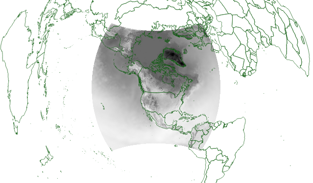
Figure 4. Here is the resulting TSOIL_aeqd.tif loaded into QGIS.
Figure 5. Here is the resulting TSOIL_aeqd.tif loaded into QGIS and zoomed-in to show that we have a good fit when compared to Natural Earth 1:10m “Admin 0 – Countries.”